Market Says 1%. Reality Delivers 0.43%. Build the Bot That Actually Knows the Difference

Cover image

I am going to break down how to build a bot that takes a pile of past outcomes and returns the one number every trade depends on: the real probability of the next event. Not a win rate. Not a gut feel. A calibrated probability with an honest confidence interval attached. I will explain every formula, show the exact code, and run the whole thing end to end on one worked example.

Let's get straight to it.

Bookmark This -> you will want the exact formulas and the estimator class the moment you point this at your own data.

Here is the development that makes this worth building right now.

In February 2026, Jonathan Becker released the largest publicly available prediction market dataset: hundreds of millions of Polymarket and Kalshi trades, every resolution outcome included, free and MIT licensed. For the first time, anyone can measure what a price actually means. And the answer, once you measure it, is uncomfortable.

A contract trading at one cent implies a one percent probability. In Becker's data, those contracts historically resolve YES only about 0.43 percent of the time. The market's own number is wrong by more than half. This is the favorite-longshot bias, and it is not a Polymarket quirk. A separate 2026 study of 292 million trades across 327,000 contracts found that calibration on these venues is a structured, multidimensional failure, with political markets chronically compressed toward fifty percent. The price is a distorted signal, and the millions of people quoting it as a probability are quoting a number that does not hold up.

That is the entire reason this bot exists. If the market number cannot be trusted, you have to compute the probability yourself, from outcomes, with the math that turns raw counts into calibrated estimates. This article is that math and that machine.

By the end of this article you will understand exactly why counting outcomes gives you the wrong probability, how the Beta-Binomial engine converts a win rate into a trustworthy estimate, how to choose the prior that controls your behavior on thin data, how to attach a confidence interval that tells you whether to bet at all, how to decide which past outcomes even count as relevant, how to prove your bot is calibrated instead of just assuming it, and how to assemble all of it into one system you can point at a dataset today.

Note: This is not a skim. Every part builds on the one before it. If you want a bot that outputs numbers you can actually size positions on, read every line.

The Method Skeleton

The whole system in eight steps. Screenshot this.

Ingest every past outcome into a structured record: a binary result plus the features of the situation it happened in.
Bucket outcomes by similar state, so you only count evidence that is actually relevant to the event you are pricing.
Count successes k and total trials n inside the matching bucket.
Estimate the probability with the Beta-Binomial posterior mean (k + α) / (n + α + β), never raw k / n.
Prior -> set α and β from a uniform default, the Jeffreys prior, or an empirical-Bayes fit on your whole dataset.
Quantify uncertainty with the credible interval from the Beta posterior. The width is your confidence.
Shrink thin buckets toward the global base rate using a hierarchical fallback, so three outcomes never masquerade as a distribution.
Calibrate with Brier score and log loss, then recalibrate if the numbers lie. Roll the posterior forward as new outcomes land.

Everything below is the detail behind those eight lines.

Prerequisites

You need Python 3.9 or higher, numpy and scipy, and a source of historical outcomes. That source can be your own logged results, or the Becker dataset (github.com/Jon-Becker/prediction-market-analysis), which ships as Parquet files you can query directly with DuckDB. You need to understand what a probability is. You do not need a statistics degree. Every formula here is defined on first use.

The one conceptual requirement: you have to accept that a probability is not a single number you observe. It is an unknown quantity you estimate, with uncertainty around it. That single shift is what separates this bot from a spreadsheet that divides wins by total.

Part 1: Why Counting Outcomes Gives You the Wrong Number

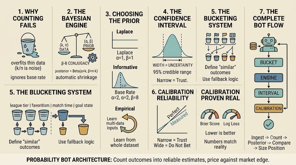
The naive way to turn outcomes into a probability is to divide. You saw the event happen k times out of n, so you call the probability k / n. This is the maximum likelihood estimate, and for large n it is fine. For the sample sizes you actually have, it fails in two specific, opposite ways.

Failure one: it overfits thin data. An underdog wins three matches out of three in your records. The naive estimate says the probability is 100 percent. That is obviously false, and yet the formula states it with total confidence. Three outcomes is not a distribution. It is noise wearing the costume of a distribution. The same thing happens at zero: a team loses five in a row and the naive estimate declares the probability is exactly zero, which no real event ever is.

Failure two: it ignores the base rate. The naive estimate uses only the handful of outcomes inside your bucket and throws away everything you know about how these events behave in general. If underdogs in general win around twenty percent of the time, a bucket showing three wins in three tries should not pull you all the way to certainty. It should update you upward from twenty percent, by an amount that depends on how much data you have.

These two failures are the bias-variance tradeoff stated in plain language. Trust the small sample too much and you get variance: wild estimates that swing on noise. Ignore the sample and lean only on the base rate and you get bias: estimates that never adapt to real signal. The naive count lives at the worst corner of this tradeoff. It is pure variance with no shrinkage.

The market itself is the proof. When you treat the crowd's implied probability as the truth, you are trusting a raw count of biased flow. Becker's data shows exactly where that breaks: at one cent, the crowd prices one percent and reality delivers 0.43 percent. The count is systematically, measurably wrong at the extremes, and it is wrong in a direction you can predict. A probability engine that does nothing but count inherits every one of those errors.

The fix is not a better count. It is a different object entirely. Instead of asking "what fraction of outcomes were wins," you ask "given these outcomes and what I already know, what is the full distribution of the true probability." That is a Bayesian question, and it has a closed-form answer that is almost suspiciously clean.

Part 2: The Bayesian Engine (Beta-Binomial Conjugacy)

Treat the unknown probability, call it θ, as a random variable with its own distribution rather than a fixed value you are trying to pin down. Before you look at any outcomes, you hold a prior distribution over θ. After you observe outcomes, you update it into a posterior distribution. The posterior is your answer.

For binary events, the natural prior is the Beta distribution, written Beta(α, β). It lives on the interval from 0 to 1, which is exactly where probabilities live. Its two parameters have a concrete meaning: α acts like a count of prior successes and β like a count of prior failures. Its mean is:

mean of Beta(α, β) = α / (α + β)

So Beta(2, 8) has mean 2 / 10 = 0.20 and encodes a belief centered on twenty percent, held with the strength of ten pseudo-observations.

The outcomes themselves follow a Binomial distribution: k successes in n independent trials, each with probability θ. Now the key result. When you combine a Beta prior with Binomial data, the posterior is again a Beta distribution, with the counts simply added in:

prior:      Beta(α, β)
data:       k successes, n − k failures
posterior:  Beta(α + k, β + n − k)

This property is called conjugacy, and it is the reason this engine is fast enough to run on every market simultaneously. Updating your entire belief about a probability is one addition. No integration, no sampling, no solver.

Your point estimate is the posterior mean:

p_bayes = (α + k) / (α + β + n)

Look at what this does to the two failure modes from Part 1. Take the underdog who won three of three, and hold the prior Beta(2, 8):

naive:      3 / 3           = 1.0000   (certainty on 3 outcomes — absurd)
bayesian:   (2 + 3) / (10 + 3) = 5 / 13 = 0.3846

The Bayesian estimate moves you from the twenty percent base rate up to about thirty-eight percent. It heard the signal, three wins is real evidence, but it refused to be dragged to certainty by three data points. That is exactly the behavior you want.

The reason it behaves this way is visible when you rewrite the posterior mean as a weighted average:

p_bayes = w · (k / n) + (1 − w) · (α / (α + β))
 
where  w = n / (n + α + β)

The estimate is a blend of the sample mean k / n and the prior mean α / (α + β). The weight w on the data grows as n grows. With few outcomes, w is small and you lean on the prior. With many outcomes, w approaches one and the data takes over. The shrinkage is automatic and it is governed entirely by how much evidence you have. You never hand-tune when to trust the sample. The arithmetic does it.

Here is the engine in code. Two functions carry the entire point estimate.

def posterior_params(k, n, alpha_prior, beta_prior):
    """Beta-Binomial conjugate update. Returns posterior (alpha, beta)."""
    return alpha_prior + k, beta_prior + (n - k)
 
def posterior_mean(k, n, alpha_prior, beta_prior):
    a, b = posterior_params(k, n, alpha_prior, beta_prior)
    return a / (a + b)

That is the whole estimator. Everything from here is about choosing the prior well, attaching uncertainty, deciding what goes into k and n, and proving the output is honest.

Part 3: Choosing the Prior

The prior is not a nuisance parameter. It is the knob that controls exactly how your bot behaves when data is thin, which is precisely when a bad estimate costs you the most. There are three defensible choices, in increasing order of sophistication.

The uniform prior: Laplace's rule of succession

Set α = 1 and β = 1. Beta(1, 1) is the uniform distribution: before any data, every probability from 0 to 1 is equally likely. The posterior mean becomes:

p = (k + 1) / (n + 2)

This is Laplace's rule of succession, and it is a strong default. It never returns exactly 0 or exactly 1, so it structurally cannot produce the certainty errors of the naive count. Three of three gives 4 / 5 = 0.80 instead of 1.00. It is gentle, assumption-free, and correct to reach for when you genuinely have no prior knowledge.

The Jeffreys prior

Set α = 0.5 and β = 0.5. Beta(0.5, 0.5) is the Jeffreys prior for a binomial proportion, and it is the standard choice in statistics when you want a prior that is uninformative in a specific technical sense, invariant under reparameterization. The posterior mean is:

p = (k + 0.5) / (n + 1)

It pulls slightly less toward the center than Laplace, so it lets small samples speak a little louder while still refusing to hit the boundaries. Use it when you want minimal shrinkage but still need the boundary protection.

The informative prior: inject what you actually know

This is the one that matters for trading, because you are never truly ignorant. You know the base rate. You may know the market's implied probability. Encode it directly. Pick a prior mean m equal to your base rate, and a prior strength s = α + β equal to the number of pseudo-observations you want that belief to be worth.

Then:

α = m · s
β = (1 − m) · s

A base rate of twenty percent held with strength ten gives α = 2, β = 8, the Beta(2, 8) from Part 2. Strength is the lever. A small s means the prior is a weak nudge that data quickly overrides. A large s means you demand a lot of evidence before you will move off your base rate. This is how you build domain knowledge into the machine without hard-coding rules.

Empirical Bayes: learn the prior from the data itself

The most powerful option is to stop guessing the prior and estimate it from your whole dataset. Look at the observed win frequency of every bucket you have, and fit a single Beta(α, β) that describes how those frequencies are distributed across buckets. Then use that fitted Beta as the prior for every individual bucket.

You fit it with the method of moments. Let m be the mean of your bucket-level frequencies and v be their variance. The Beta parameters that produce that mean and variance are:

s = m · (1 − m) / v − 1
α = m · s
β = (1 − m) · s

valid whenever v < m · (1 − m). This is empirical Bayes: the prior is no longer an assumption, it is a measurement of how probabilities are actually distributed in your domain. A bucket with little data gets pulled toward the behavior of buckets in general, which is exactly the right thing to do when a bucket has not earned an opinion of its own yet.

def fit_empirical_bayes(bucket_frequencies):
    """Method-of-moments Beta fit across observed bucket win rates."""
    import numpy as np
    m = np.mean(bucket_frequencies)
    v = np.var(bucket_frequencies)
    if v <= 0 or v >= m * (1 - m):
        return 1.0, 1.0                      # fall back to uniform
    s = m * (1 - m) / v - 1
    return m * s, (1 - m) * s

To be clear about which to use: start with Laplace while you are building, switch to an informative prior once you have a real base rate, and move to empirical Bayes once you have enough buckets to fit one. Each step makes the bot's thin-data behavior more honest.

Part 4: The Confidence Interval That Tells You Whether to Trust the Number

A point estimate alone is dangerous, because 26 percent computed from 5 outcomes and 26 percent computed from 5,000 outcomes are not the same claim, even though the number is identical. The difference is uncertainty, and the Bayesian engine hands it to you for free, because your answer is a full distribution, not a point.

The credible interval is the range that contains the true probability with a stated posterior probability, typically 95 percent. You read it straight off the posterior Beta by taking its 2.5th and 97.5th percentiles:

from scipy import stats
 
def credible_interval(k, n, alpha_prior, beta_prior, level=0.95):
    a, b = alpha_prior + k, beta_prior + (n - k)
    lo = (1 - level) / 2
    hi = 1 - lo
    return stats.beta.ppf(lo, a, b), stats.beta.ppf(hi, a, b)

The width of this interval is the single most important output of the bot after the point estimate. A narrow interval means the data has spoken clearly and you can act. A wide interval means you do not know enough to bet, no matter how attractive the midpoint looks. This is the formal version of the rule every systematic trader eventually learns the hard way: a thin bucket is not tradeable. The interval turns that instinct into a number.

If you prefer a frequentist interval, use the Wilson score interval rather than the textbook normal approximation. The normal approximation, p ± z · sqrt(p(1−p)/n), is the Wald interval, and it is badly wrong for small n or extreme p. It can produce bounds below zero or above one, and it collapses to zero width when k is zero. The Wilson interval fixes both. For z = 1.96 at 95 percent:

center     = (p + z² / (2n)) / (1 + z² / n)
half-width = z / (1 + z² / n) · sqrt( p(1−p)/n + z² / (4n²) )

where p = k / n. It stays inside the valid range and stays sensible at the extremes.

The interval is also the hook into position sizing. In my earlier breakdown of empirical Kelly, the sizing formula haircuts the Kelly fraction by the coefficient of variation of your edge estimate, f_empirical = f_kelly · (1 − CV_edge). The width of this credible interval, relative to the estimate, is a direct measure of that uncertainty. Wide interval, large haircut, smaller position. The interval does not just tell you whether to bet. It tells you how much.

Part 5: Defining "Similar" -> The Bucketing System

The engine in Parts 2 through 4 is only as good as the outcomes you feed it. If you count outcomes that are not actually relevant to the event you are pricing, you get a precise estimate of the wrong thing. So the real design problem is this: which past outcomes count as evidence for the next one?

The answer is bucketing. You describe the situation an outcome occurred in using a set of features, discretize each feature into a small number of levels, and combine them into a bucket key. Two outcomes share a bucket only when their situations match across every feature. Then you count k and n inside the bucket that matches the event you are pricing.

This is the same idea I used to classify shocks in the World Cup strategy: league tier, favoritism, order book depth, match time, goal state, concatenated into one key. Generalize it. Pick features that plausibly change the outcome, cut each into levels, and join them.

def bucket_key(record):
    return "|".join([
        classify_tier(record.league),        # major | minor
        classify_favoritism(record.price),   # heavy | moderate | slight | underdog
        classify_time(record.minute),        # early | mid | late | final
        classify_state(record.goal_diff),    # level | close | comfortable | blowout
    ])
# e.g. "major|underdog|mid|level"

Bucketing has its own bias-variance tradeoff, and it is the mirror image of the one from Part 1. Add more features and each bucket becomes a more exact description of the situation, but the outcomes get spread thinner across more buckets, so n per bucket falls and variance rises. Use fewer features and every bucket holds more data, but the description is coarser and you blur genuinely different situations together, which raises bias. This is the same square-root-of-N logic that governs combining independent signals: more conditioning dimensions help only up to the point where each bucket still has enough data to mean something.

The way to get both is a hierarchical fallback. Define your buckets at several levels of coarseness. When the full, most-specific bucket has enough outcomes, use it. When it is too thin, back off to a coarser bucket by dropping the least important feature, and shrink the specific estimate toward the coarse one. This is partial pooling, and it is exactly the structure the 2026 calibration study used, a Bayesian hierarchical model, to show that calibration is real but domain-dependent. You borrow strength from the general when the specific has not earned its own opinion, and you let the specific take over as it accumulates evidence.

def estimate_with_fallback(record, index, min_trials=8):
    """Walk from most specific bucket to coarsest until one has enough data."""
    for key in bucket_hierarchy(record):        # specific -> coarse
        k, n = index.counts(key)
        if n >= min_trials:
            return key, k, n
    k, n = index.global_counts()                # base rate as final backstop
    return "GLOBAL", k, n

The min_trials threshold is where you draw the line between "enough data to trust this bucket" and "fall back." It is the same discipline as refusing to build a distribution from three shocks. Set it deliberately.

Part 6: Calibration -> Proving the Numbers Are Real

Everything so far produces probabilities. This part is how you prove those probabilities are honest, because an estimator that outputs numbers is worthless if the numbers do not correspond to reality. A probability is calibrated when it matches observed frequency: of all the times your bot said thirty percent, the event should happen about thirty percent of the time. If it happens fifteen percent of the time, your bot is overconfident and every position sized on it is wrong.

You measure calibration three ways, and you run all three continuously.

The reliability diagram

Bin your predictions into ranges, then within each bin compare the average predicted probability to the actual frequency of the event. Plot predicted on one axis, realized on the other. A perfectly calibrated bot traces the diagonal. Systematic deviation above or below the line is systematic bias you can see and correct. This is the exact instrument that exposes the favorite-longshot bias in market prices, and you point it at your own bot to catch the same disease in yourself.

The Brier score

The Brier score is the mean squared error of probabilistic predictions. For predictions p_i and outcomes o_i in {0, 1}:

Brier = (1 / N) · Σ (p_i − o_i)²

Lower is better; zero is perfect. It rewards being both correct and confident, and it decomposes cleanly into a calibration term and a resolution term, so a rising Brier score tells you your edge is decaying before your P&L does.

Log loss

Log loss punishes confident wrong predictions far more harshly than the Brier score does:

LogLoss = − (1 / N) · Σ [ o_i · ln(p_i) + (1 − o_i) · ln(1 − p_i) ]

A prediction of 0.99 that resolves the wrong way contributes an enormous penalty. If your bot is going to be confidently wrong, log loss is the metric that will scream about it first. Track both: Brier for overall quality, log loss for tail risk in your confidence.

import numpy as np
 
def brier_score(p, o):
    p, o = np.asarray(p), np.asarray(o)
    return np.mean((p - o) ** 2)
 
def log_loss(p, o, eps=1e-15):
    p, o = np.clip(p, eps, 1 - eps), np.asarray(o)
    return -np.mean(o * np.log(p) + (1 - o) * np.log(1 - p))

If the reliability diagram shows your bot is miscalibrated in a consistent way, you fix it with a recalibration map fit on held-out data: Platt scaling, which fits a logistic transform from your raw output to a calibrated one, or isotonic regression, which fits a monotonic step function and assumes less about the shape. Fit it once on a validation set, apply it to every future prediction. This is the loop that turns a plausible estimator into a trustworthy one, and it is the step almost everyone skips.

Part 7: The Complete Bot (Architecture and Worked Example)

The full system has four components. A data layer ingests outcomes and builds a bucket index of k and n at every level of the hierarchy. A prior layer fits the empirical-Bayes Beta once across all buckets. An estimation layer takes a query, walks the bucket fallback, and returns the posterior mean plus the credible interval. A calibration layer logs every prediction against its eventual outcome and reports Brier and log loss so you know the moment the edge starts to rot.

Here is the estimator as one class.

import numpy as np
from scipy import stats
 
class ProbabilityBot:
    def __init__(self, alpha_prior=1.0, beta_prior=1.0, min_trials=8):
        self.alpha, self.beta = alpha_prior, beta_prior
        self.min_trials = min_trials
 
    def fit_prior(self, bucket_frequencies):
        m, v = np.mean(bucket_frequencies), np.var(bucket_frequencies)
        if 0 < v < m * (1 - m):
            s = m * (1 - m) / v - 1
            self.alpha, self.beta = m * s, (1 - m) * s
 
    def estimate(self, k, n, level=0.95):
        a, b = self.alpha + k, self.beta + (n - k)
        mean = a / (a + b)
        lo = stats.beta.ppf((1 - level) / 2, a, b)
        hi = stats.beta.ppf(1 - (1 - level) / 2, a, b)
        return {"prob": mean, "low": lo, "high": hi,
                "width": hi - lo, "n": n}
 
    def edge(self, k, n, market_price):
        est = self.estimate(k, n)
        est["edge"] = est["prob"] - market_price
        est["tradeable"] = est["width"] < 0.20        # your discipline knob
        return est

Now run it start to finish on one real scenario.

You are pricing whether an underdog wins a match. You pull the matching bucket from your index, major | underdog | mid | level, and it holds 28 historical outcomes, of which the underdog won 8. Your base rate for underdogs in this bucket family is twenty percent, so your prior is Beta(2, 8).

Step 1, the naive number. 8 / 28 = 0.2857. Twenty-nine percent, stated with false confidence.

Step 2, the posterior. With the Beta(2, 8) prior, the posterior is Beta(2 + 8, 8 + 20) = Beta(10, 28), and the posterior mean is 10 / 38 = 0.2632. Twenty-six percent. The estimate shrank from the naive 28.6 percent toward the twenty percent base rate, because 28 outcomes is real but not overwhelming. The data weight here is w = 28 / 38 = 0.737, so the estimate is 74 percent data, 26 percent prior.

Step 3, the interval. The 95 percent credible interval from Beta(10, 28) runs from 0.138 to 0.412, a width of 0.274. For contrast, the naive Wald interval would run from 0.118 to 0.453, wider and partly built on the false-confidence point. The interval is wide enough that you know this is a moderate-conviction estimate, not a lock.

Step 4, the edge. The market is pricing YES at 0.22. Your estimate is 0.2632. The edge is +0.043, about four cents of expected value in your favor. The credible interval does not exclude the market price, so this is a lean, not a hammer. You size it small, and empirical Kelly haircuts it further for the interval width. You do not back up the truck on a four-cent edge with a twenty-seven-point interval, and now you have the numbers that say so explicitly.

Step 5, the discipline check. Compare that to the thin-bucket trap. If this bucket had held only 3 outcomes at 3 wins, the naive number would be 100 percent, the Bayesian estimate would be 38 percent, and the credible interval would run from 0.15 to 0.65, a width of 0.50. Half the probability line. The bot would flag it as untradeable on width alone, and it would be right. Same math, and it saves you from the single most common way these systems blow up.

That is the entire loop. Ingest outcomes, bucket them, count, estimate with the posterior, attach the interval, compare to the market, size by the width. Repeat across every event you care about.

Common Mistakes

The failures are predictable, so name them in advance.

Trusting raw k / n on a thin bucket is the original sin, and everything in Part 2 exists to prevent it. Over-bucketing until every bucket holds one or two outcomes recreates the same problem from the other direction, and Part 5's fallback is the cure. Using a flat prior when you have a real base rate throws away free information, so move to an informative or empirical-Bayes prior as soon as you can fit one. Never checking calibration means you are flying blind on whether your numbers mean anything, and Part 6 is not optional. Reading the point estimate while ignoring the interval leads you to bet the same size on a five-outcome guess and a five-thousand-outcome near-certainty. Leaking the outcome you are predicting into the bucket that defines the estimate is a look-ahead bug that makes your backtest glow and your live results collapse. And treating old outcomes as equal to recent ones ignores that regimes change; weight recent data more heavily or decay old outcomes when the process is non-stationary.

The Summary

A win rate is a count. A probability is a distribution. The whole job of this bot is to convert the first into the second without lying to you about how much it knows.

The Beta-Binomial engine does the conversion in one addition, because a Beta prior updated by Binomial outcomes stays a Beta, and its mean (k + α) / (n + α + β) is a self-weighting blend of your data and your prior. The prior controls thin-data behavior, and empirical Bayes lets you learn it from the data instead of guessing. The credible interval turns uncertainty into a number you can size on, and it is the difference between a tradeable estimate and a coin flip in a costume. Bucketing decides which outcomes count, with a hierarchical fallback so the specific borrows strength from the general until it earns its own opinion. And calibration, measured with Brier score and log loss on a live reliability diagram, is how you prove the numbers correspond to reality instead of assuming they do.

The market's own probability fails this test in public: one-cent contracts that resolve at 0.43 percent are a count that never became a calibrated estimate. Build the bot that does the step the market skips, and you are pricing with the true distribution while everyone else is quoting a broken number.

Here is the question I want you to sit with.

Your bot outputs 26 percent with a credible interval from 14 to 41. The market says 22. The edge is real but the interval swallows it. Do you take the trade because the midpoint has an edge, or do you pass because the interval says you do not actually know? Your answer is the entire difference between a probability engine and a random number generator with good manners.

There is no wrong answer. But there are very revealing ones.